


In mathematics, a rate of change is a mathematical expression that relates changes in one quantity to changes in another quantity. Rates of change are useful for describing how systems change over time and how a change in one variable affects change in another. Rates of change are useful is a number of fields where they are used to summarize a relationship between two variables.
A simple example of a rate of change is velocity. At its core, velocity is a rate of change. Specifically, velocity describes a change in distance with respect to a change in time. A velocity of 3 m/s tells us that the displacement of an object is changing by 3 meters for every 1 second. For every change in the independent variable (time) the dependent variable (distance) changes by 3 meters.
Rates of change are particularly useful in algebra, calculus, and physics as those fields routinely deal with complex systems where continuous changes in one variable correlate with changes in another. Rates of change allow us to describe and predict how two quantities change with respect to each other.
Rate Of Change Formula
At its simplest, the rate of change of a function over an interval is just the quotient of the change in the output of a function (y) over the difference in the input of the function (x) (change in y/change in x)
![]()
More specifically, for any function ƒ(x), the average rate of change of that function over the interval a ≤ x ≤ b is just:
![]()
The rate of change over an interval is a measure of how much the output of a function changes per unit of input over that interval.
Let’s return to the example of velocity to see exactly how you can calculate a rate of change. Here is a table describing the distance a car covers over some given time:
| Time (seconds) | Distance Traveled (meters) |
| 0 | 0 |
| 1 | 2 |
| 2 | 4 |
| 3 | 6 |
| 4 | 8 |
| 5 | 10 |
The table tells us that at t=1, the car has moved 2 meters, at t=2 the object has moved 4 meters, at t=3 6, at t=4 8, and at t=5 10 meters. We want to figure out the rate of change of the car’s displacement over time over the interval 0 to 5 seconds. The average rate of change can be found by dividing the change in distance by the change in time:
rate of change = Δdistance/Δtime
rate of change = (10-0)/(5-0) = 20/5 = 2 m/s
The average velocity of the object is 2 m/s, meaning that for every second of time that passes, the distance traveled by the car changes by 2 meters. This is why velocity is a rate of change: it tells us how one variable (distance) changes with respect to change in another variable (time). We can use this data to predict how far the car will travel in the future. Assuming the rate of change (velocity) remains constant, after 6 seconds the car will have traveled 12 meters, after 7 seconds 14 meters, and so on.
Graphs And Rates Of Change
Graphing data points can be helpful for visualizing rates of changes. Taking our time-distance data points from the last section and placing it on an x-y coordinate axis with time on the x-axis and distance on the y-axis gives us:

Credit: Author. Generated using GraphFree.
Plotting our data points creates a nice line. Looking at the shape of the graph highlights an important principle. The slope of a particular graph gives us important information about the rate of change of a function.
Recall that the slope of a graph between two points is equal to the change in the y-variable divided by the change in the x-variable. The slope of a graph tells us the rate of change of the output (y) of the graph with respect to changes in the input (x). For example, the slope of the graph between (1, 2) and (2, 4) can be discovered by the same formula:
slope = Δy/Δx (“rise”/”run”)
slope = (4−2)/(2−1) = 2
The slope of the graph is 2 meaning the rate of change between the two points (1, 2) and (2, 4) is 2. The slope of the function corresponds to how “steep” the line on the graph is. The larger the slope, the steeper the line between the two points, the smaller the slope the less steep. If the slope is negative then the rate of change is also negative. For example, say our car starts 10 meters away, and starts moving towards you:
| Time | Distance |
| 0 | 10 |
| 1 | 8 |
| 2 | 6 |
| 3 | 4 |
| 4 | 2 |
| 5 | 0 |
What is the rate of change of these data points? Using our formula, we can calculate:
rate of change = Δy/Δx
rate of change = (0−10)/(5−0) = −2
In this case, the rate of change is −2. This means that the y-value (distance) is changing by −2 for every unit of time. Graphing these data points gives us:
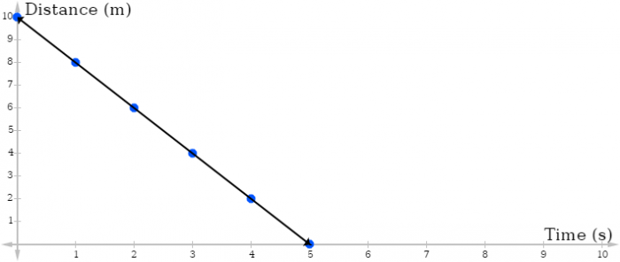
Since the rate of change is negative, the graph slopes downwards to the right. The general shape of a graph can tell you general information about the rate of change of the function. If it slopes upwards to the right, then the rate of change is positive. If it slopes downwards to the right, then the rate of change is negative. Whether the rate of change is positive or negative tells us whether the output increases or decreases with respect to changes in the input.
Non-Constant Rate Of Change
So far, the examples we have looked at involve a constant rate of change; i.e. the change in the output of the function is constant over every interval. In our previous examples with velocity, the rate of change between each point in time is the same, 2 m/s. Every second the cars distance changes by a constant amount.
What about cases where the rate of change between each point of the function is not constant? Say the data points for our moving car instead look like this:
| Time (s) | Distance (m) |
| 0 | 0 |
| 1 | 1 |
| 2 | 4 |
| 3 | 9 |
| 4 | 16 |
| 5 | 25 |
Notice that between each point in time, the rate of change is different. From t=0 to t=1 seconds, the rate of change is (1−0)/(1−0) = 1 but from t=1 to t=2 the rate of change is (4−1)/(2−1) = 3. From t=2 to t=3, the rate of change is (9−4)/(3−2) = 5 and from t=3 to t=4, the rate of change is(16−9)/(4−3) = 7. At each point in time, the rate of change of the function is increasing, meaning that over time the car is accelerating. Graphing these data points gives us this shape:
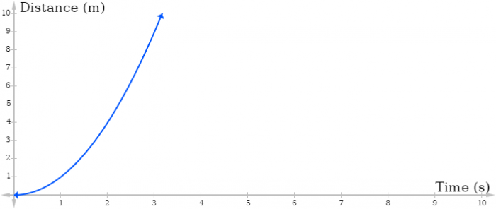
Because the rate of change is not constant, the graph does not look like a straight line but instead takes on a curved shape. The curve of the line tells not only that the rate of change is positive (it slopes up to the right) but also that the rate of change is increasing over the interval. The steeper the line between two points of the graph, the greater the rate of change between those two points are. Notice how as time goes on, the graph gets steeper and steeper. The increasing steepness of the graph corresponds to an increasing rate of change. Consequently, if the graph began at the top and sloped downward, that would indicate that the rate of change is increasing in the negative direction.
Rate Of Change Practice Problems
Q1.) The displacement of a car with respect to time is given by the following table:
| Time (s) | Displacement (m) |
| 0 | 5 |
| 1 | 2 |
| 2 | 10 |
| 3 | 15 |
| 4 | 12 |
(i) What is the average rate of change of the displacement from the interval t=0 to t=4? (ii) What is the average rate of change between t=0 and t=1?
Answer: Using our rate of change formula, we can figure out that the average rate of change over the interval t=0 to t=4 is equal to:
rate of change = Δy/Δx
rate of change = (12−5)/(4−0) = 7/4.
(i) The average rate of change of the car’s displacement over time is 7/4
For (ii) we need to figure out the rate of change between t=0 and t=1. These values are:
rate of change = (2−5)/(1−0) = −3
The average rate of change between t=0 and t=1 is −3, meaning that displacement is decreasing between those two points in time.
Q.2) The vertical height of a projectile in freefall is given by the equation: d = ½gt2 where g is the acceleration due to gravity (on Earth, g = −9.8 m/s2). If a cannonball is dropped off the leaning tower of Pisa, how far in meters will it fall in 3.4 seconds? What is the average velocity of the cannonball from t=1 to t=3?
We know that when t=0, the vertical height of the cannonballs is also 0 (because it has not been dropped yet). To find how much the displacement has changed in 3.4 seconds, we need to find the vertical height after 3.4 seconds have passed. Using the freefall equation, we know that after 3.4 seconds, the cannonball will have dropped:
d = ½(−9.8)(3.4)2
d = −56.4 meters. (the answer is negative because the cannonball is moving down)
After 3.4 seconds, the cannonball will have fallen 56.4 meters.
To find the average velocity of the cannonball from t=1 to t=3, we have to find the displacement of the cannonball at each of those points. At t=1, the cannonball has fallen:
d = ½(−9.8)(1)2
d = −4.9 meters.
After 1 second has passed, the cannonball has fallen 4.9 meters. At t=3:
d = ½(−9.8)(3)2
d = −44.1 meters
After three seconds the cannonball will have fallen 44.1 meters. Thus the average velocity of the cannonball from t=1 to t=3 is:
rate of change = (−44.1−−4.9)/(3−1) = −19.6 m/s
Between the times t=1 and t=3, the cannonball has an average velocity of −19.6 m/s.
Related Posts
 Improving Tools For Quality Improvement: Crossings, Runs, And Crossrun
 Coherent Poly Propagation Materials With 3-Dimensional Photonic Control Over Visible Light
 Reconstructing Commuter Networks Using Machine Learning And Urban Indicators
 Surprising Internal Structure Of Whole Wheat-Green Gram Functional Bread
 Tailoring Tomatoes To Match Individual Consumer Needs
 Eavesdropping On “Classroom Talk” In Undergraduate STEM Classrooms