How To Find Horizontal Asymptotes

A horizontal asymptote is a horizontal line on a graph that the output of a function gets ever closer to, but never reaches. In more mathematical terms, a function will approach a horizontal asymptote if and only if as the input of the function grows to infinity or negative infinity, the output of the function approaches a constant value c. Symbolically, this can be represented by the two limit expressions:

Essentially, a graph of a function will have a horizontal asymptote if the output of the function approaches some constant as x grows arbitrarily large in the positive or negative direction. If either of the above expressions are true, then a graph of the function will have a horizontal asymptote at the line y=c. An example is the function ƒ(x)=(8x²-6)/(2x²+3). Plotting the graph of this function gives us:

This rational function has a horizontal asymptote at y=4. Notice how as the x value grows without bound in either direction, the blue graph ever approaches the dotted red line at y=4, but never actually touches it.  Other kinds of asymptotes include vertical asymptotes and oblique asymptotes. Any rational function has at most 1 horizontal or oblique asymptote but can have many vertical asymptotes.

A horizontal asymptote can be defined in terms of derivatives as well. In a nutshell, a function has a horizontal asymptote if, for its derivative, x approaches infinity, the limit of the derivative equation is 0. This corresponds to the tangent lines of a graph approaching a horizontal asymptote getting closer and closer to a slope of 0

There are some simple rules for determining if a rational function has a horizontal asymptote. But to understand them we first need to take a look at the idea of the degree of a polynomial.

Degree Of A Polynomial

A polynomial is an expression consisting of a series of variables and coefficients related with only the addition, subtraction, and multiplication operators. The general form of a polynomial is

axⁿ+by^m  

where a and b are constant coefficients, x and y are variables (sometimes called indeterminates), and n and m are some non-negative integers. So for instance, 3x²+4x-6 is a polynomial expression as it consists of a combination of coefficients and variables connected by the addition operator. Likewise, 9x⁴-3xz³+7y² is also a polynomial with three separate variables.

The degree of a polynomial can be determined by adding together the degrees of its individual monomial terms. The degree of a term is equal to the sum of the exponents superscripts of the variable(s) in one monomial term. The degree of an entire polynomial is equal to the highest degree of its individual monomial terms.

For instance, the polynomial 4z⁴x³−6y³z²+2xz-7, which can be written as 4x⁴y³−6x³y²+2x¹y¹-7x⁰y⁰, has 4 terms. The first term 4z⁴x³ has a degree of 7 (3+4), the second term 6x³y² has a degree of 5 (3+2), the third term 2x¹y¹ a degree of 2 (1+1) and the fourth term 7x⁰y⁰ a degree of 0 (0+0). Since 7 is the monomial term with the highest degree, the degree of the entire polynomial is 7.

Rules For Finding Horizontal Asymptotes

Now that we have a grasp on the concept of degrees of a polynomial, we can move on to the rules for finding horizontal asymptotes. Whether or not a rational function in the form of R(x)=P(x)/Q(x) has a horizontal asymptote depends on the degree of the numerator and denominator polynomials P(x) and Q(x).

The general rules are as follows:

• If degree of top < degree of bottom, then the function has a horizontal asymptote at y=0. In the function ƒ(x) = (x+4)/(x²-3x), the degree of the denominator term is greater than that of the numerator term, so the function has a horizontal asymptote at y=0.
• If degree of top = degree of bottom, divide the coefficients of the highest degree terms. For example in the function ƒ(x)=(8x²-6)/(2x²+3), the degree of both the top and bottom polynomials is 2. dividing the coefficients of the highest degree terms gives 8/2=4. So the function has a horizontal asymptote at y=4.
• If degree of top > degree of bottom, then the function does not have a horizontal asymptote. ƒ(x) = (2x²)/(x-5) does not have any horizontal asymptote because the degree of the numerator polynomial is greater than that of the denominator polynomial.

In special cases where the degree of the numerator is greater than the denominator by exactly 1, the graph will have an oblique asymptote.

As with all things related to functions, graphing an equation can help you determine any horizontal asymptotes. Though graphing is not a way to prove that a function has a horizontal asymptote, it can be helpful and point you in the right direction for finding one.

Problems With Solutions

Let’s look at some problems to get used to these rules for finding horizontal asymptotes.

Find the horizontal asymptotes (if any) of the following functions:

1. ƒ(x)=(3x²-5)/(x²-2x+1)
2. ƒ(x)=(x²-9)/(x+1)
3. ƒ(x)=(x-12)/(2x³+5x-3)
4. ƒ(x)=(3x³+3x)/(2x³-2x)

Solutions:

(1)

For ƒ(x)=(3x²-5)/(x²-2x+1) we first need to determine the degree of the numerator and denominator polynomials. Both the top and bottom functions have a degree of 2 (3x² and x²) so dividing the coefficients of the leading terms gives us 3/1=3. So the function ƒ(x)=(3x²-5)/(x²-2x+1) has a horizontal asymptote at y=3. Graphing this function gives us:

Indeed, as x grows arbitrarily large in the positive and negative directions, the output of the function ƒ(x)=(3x²-5)/(x²-2x+1) approaches the line at y=3. Notice that this graph crosses its horizontal asymptote at one point before infinitely approaching it.

(2)

For ƒ(x)=(x²-9)/(x+1), we once again need to determine the degree of the top and bottom terms. The degree of the top is 2 (x²) and the degree of the bottom is 1 (x). Since the degree of the numerator is greater than that of the denominator, this function has no horizontal asymptotes. Indeed, graphing the function ƒ(x)=(x²-9)/(x+1) gives us:

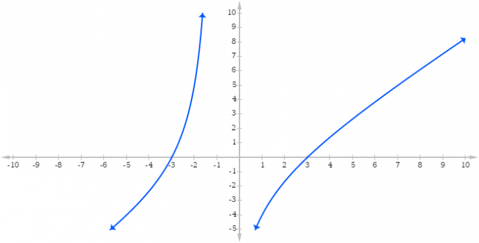
As we can see, there is no horizontal line that this graph approaches. This graph does, however, have an oblique asymptote, as the difference in degree of the top and bottom is exactly 1 (it also has a vertical asymptote at x=-1)

(3)

For ƒ(x)=(x-12)/(2x³+5x-3), the degree of the top is 1 (x) and the degree of the bottom is 3 (x³). Since the degree on the top is less than the degree on the bottom, the graph has a horizontal asymptote at y=0. Once again, graphing this function gives us:

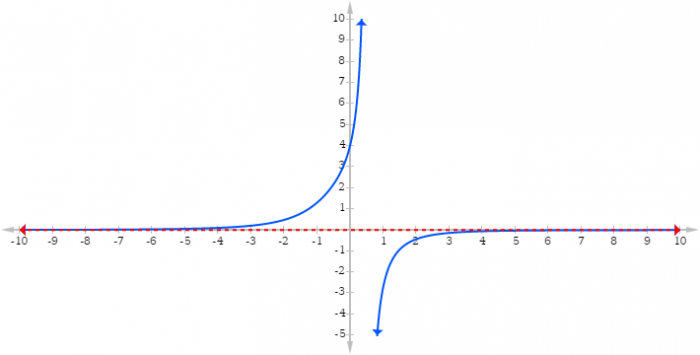
As the value of x grows very large in both direction, we can see that the graph gets closer and closer to the line at y=0.

(4)

For ƒ(x)=(3x³+3x)/(2x³-2x), we can plainly see that both the top and bottom terms have a degree of 3 (3x³ and 2x³). AS the degree of both top and bottom are equal we divide the coefficients of the leading terms to get 3/2. So the graph has a horizontal asymptote at the line y=2/3. Graphing this function gives us:
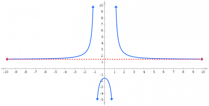We can see that the graph approaches a line at y=2/3. As the x values get really, really big, the output gets closer and closer to 2/3. This function also has 2 vertical asymptotes at -1 and 1.

Real World Examples Of Horizontal Asymptotes

Asymptotes, in general, may seem like just a mathematical curiosity. After all, the limits and infinities associated with asymptotes may not seem to make sense in the context of the physical world. However, asymptotic reasoning is common in the sciences and functions that contain asymptotes are used to model various processes or relations between quantities.  Very often, processes that tend towards some sort of equilibrium value can be modeled using horizontal asymptotes.

For example, say we are dissolving some solute into a solvent. For any given solvent, relative to some solute, there is a maximum amount of solute that the solvent can dissolve before the solvent becomes completely saturated. Once the solvent is completely saturated with solute, the solvent will not dissolve any more solute.

Plotting the amount of solute added on the x-axis against the concentration of the dissolved solute on the y-axis will show that as the amount of solute increases (x-value) the total concentration of the dissolved solute (y-value) increases, until it reaches some critical concentration, after which the concentration (y-value) will not increase anymore. This graph will have a horizontal asymptote at that line, which is equal to a concentration that is the saturation point of the solvent. The exact numerical specifics will depend on the chemical character of the solvent and solute, but for any solvent and solute, there is some point where the solute is maximally concentrated and will not dissolve anymore.

Likewise, modeling the rates of the diffusion of fluids often involve asymptotic reasoning. As time increases, a gas will diffuse to equally fill a container. Initially, the gas begins at a very high concentration, which begins to fall as the gas spreads out in the chamber. Eventually, the gas molecules will reach a point where they are as evenly distributed through the container as possible, after which the concentration cannot drop anymore. Graphing time on the x-axis and the concentration on the y-axis will give you a nice curve that begins at a high concentration, falls slowly, then eventually approaches some horizontal asymptote at some critical concentration value—the point at which the gas is completely evenly spread out in the container.