Learning In The Brain And Machines

The capacity to adapt and learn with experience is one of the most intriguing features of the brain. The recent dramatic success of artificial intelligence is indeed based on computational models  — deep neural networks — that have a structure and learning mechanisms inspired by the brain’s architecture and plasticity.

Interestingly, research on the brain shows that its learning capabilities have a key feature that is little understood from a computational point of view and generally not employed in artificial neural networks: the dependence on the timing of neural events. This review presents an article proposing a general learning rule that can be used to model the brain’s plasticity or in artificial neural networks based on such timing.

Plasticity in the brain

Neurons in the brain speak to each other on the basis of spikes. These are short-peaked changes of the electric potential that last for few milliseconds and are interleaved with several milliseconds of silence. Research has now soundly shown that learning in the brain, consisting of the change of the signal-communication strength of the physical links between pairs of neurons, depends on the timing of each pair of spikes involving the pre-synaptic neuron and the post-synaptic neuron (the links are called synapses; or connection weights in the jargon of artificial neural networks). This timing is so important that brain plasticity is often called spike-timing dependent plasticity (STDP).

Research on STDP shows that the brain uses a surprisingly wide variety of learning mechanisms. In particular, the spike-dependent change of synapses varies for excitatory neurons and inhibitory neurons, or for different areas of the brain. For example, if an excitatory pre-synaptic neuron in the brain hippocampus fires a spike few milliseconds before a spike of another excitatory neuron in the same area, the synapse between them might increase for a certain amount; instead, the synapse might decrease if the pre-synaptic neuron fires few milliseconds after the post-synaptic neuron. Other neurons might instead show a mirror decrease-increase pattern for such inter-spike intervals. The graph that plots the synaptic change corresponding to the different inter-spike intervals represents the learning kernel and is an effective way to describe a particular STDP phenomenon (see figures below).

Limitations of current computational models to capture plasticity

Very often in brain modeling, the STDP kernels are reproduced with a mathematical function (e.g., an exponential function) directly linking the synaptic change to the inter-spike interval. These phenomenological models are very simple but do not reproduce the mechanisms causing the synapse change. On the other hand, biophysical models reproduce particular STDP phenomena by capturing in great detail their electrical/chemical underlying causes, but they do this at the cost of leading to a different model for each different STDP phenomenon.

A third class of models is based on the general Hebb learning principle that can be summarised as neurons that fire together wire together. These models are at an intermediate level of complexity with respect to phenomenological and biophysical models as on one side they represent how neuron activations cause the synaptic change and on the other they abstract over biological details. Commonly, Hebb learning rules consider only one instant of time and update the synapse with functions of the co-occurrence of the activation of the pre- and post-synaptic neurons.

A less known class of Hebb learning mechanisms, called Differential Hebbian Learning (DHL) rules, instead update the synapse by taking into account the temporal relation between the changes of the activation of neurons in time. These changes are mathematically captured through first-order derivatives of the activation of neurons with respect to time. DHL rules have the potential to mimic STDP, but they can be also applied to any type of neural change beyond spike-like changes and so they might be very important for artificial neural networks. Despite this potential, few DHL rules have been proposed so far. These rules can produce only a subset of possible synaptic changes depending on the spike-interval, and so they can capture only a small subset of the STDP kernels found in the brain.

A new computational model: General Differential Hebbian Learning (G-DHL)

Recently, in our recent article titled General differential Hebbian learning: Capturing temporal relations between events in neural networks and the brain, published in the journal Plos Computational Biology, we proposed a systematization of DHL rules based on a General Differential Hebbian Learning (G-DHL) rule (all figures reported here are from the paper). To this purpose, we first highlighted how it is important to separate the DHL rule formulas from the filtering operations applied to neural signals before the application of the rules. These filtering operations can be applied to any (neural) signals to detect the changes of interest, for example when the pre-synaptic neuron activation decreases and the post-synaptic neuron increases. The filters allow the production of two new signals presenting an event in correspondence to each change of interest. An event is a transient monotonic signal increase followed by a transient monotonic signal decrease on which DHL rules can work (Figure 1). The G-DHL rule can then be applied to the two resulting “event-signals”.

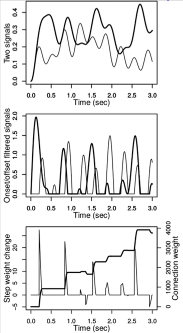
Figure 1. Top: two possible noisy signals. Middle: the event-signals obtained with two filters applied respectively to the two signals at the top: the first filter associates an event to each original signal increase; the second filter associates an event to each original signal decrease. Bottom: example of synapse change obtained by applying a rule based on the fifth and sixth components of G-DHL (see below). Image published with permission from PLOS from https://doi.org/10.1371/journal.pcbi.1006227

The G-DHL rule has a composite structure; in particular, it is formed by a linear combination of 8 components (9 if one includes the Hebb rule as a special case). These components are the possible combinations of three elements of the pre- and post-synaptic event-signals: the events; the positive part of the time-derivative of events; and the negative part of the time-derivative of events (Figure 2).

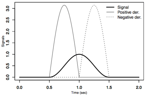
Figure 2. The three key elements needed to apply the G-DHL. Image published with permission from PLOS from https://doi.org/10.1371/journal.pcbi.1006227

The rule is quite simple, so we can report it here:

where ŵ is the synaptic change at an instant of time, σ and η are numerical coefficients each multiplying one of the eight components of the rule, u₁ and u₂ are the activations of respectively the pre- and post-synaptic neurons, ů₁ and ů₁ are their first time-derivatives in time, [x]⁺ is the positive-part function of x (i.e.: [x]⁺=x if x>0 and [x]⁺=0 if x≤0) and [x]^– is the negative-part function of x (i.e.: [x]^–=-x if x≤0, and [x]^–=0 if x>0). A nice feature of the G-DHL rule is that the components of the rule form nice non-overlapping learning kernels (Figure 3) that suitably mixed with the coefficients of the rule linear combination are able to generate all known DHL rules and many new ones. The linear nature of the rule also facilitates the manual tuning of its parameters or their estimation with automatic search algorithms.

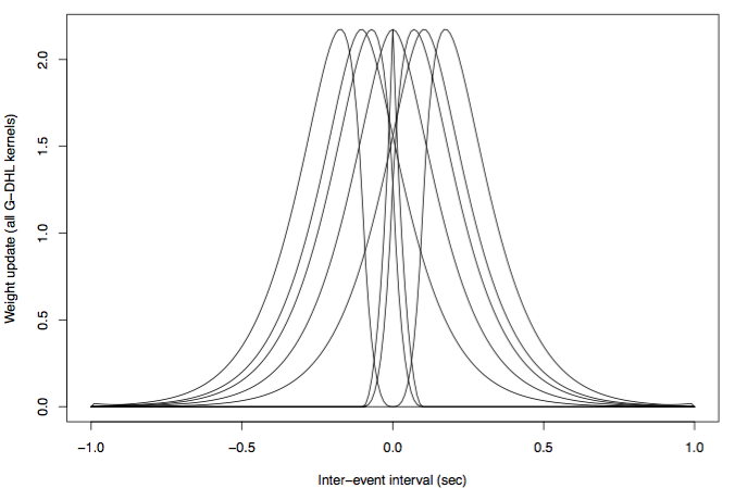
Figure 3. The eight kernels of the G-DHL rule. Y-axis: change of the synapse. X-axis: pre-/post-synaptic inter-spike interval. When a kernel is multiplied by a positive or negative coefficient within the rule it respectively produces a synapse enhancement or depression. Image published with permission from PLOS from https://doi.org/10.1371/journal.pcbi.1006227

The flexibility of the G-DHL rule

The flexibility of the G-DHL rule is shown by applying it to successfully fit, with a non-linear regression, several different STDP kernels found in the brain and analyzed in the important review of Caporale and Done (2008) (Figure 4). To this purpose, we also derived the equations that allow the closed-form computation of the synaptic change yielded by the G-DHL kernels given a certain inter-spike interval; (b) a software that uses such equations to automatically find the G-DHL components and parameters that best fit a target STDP dataset.

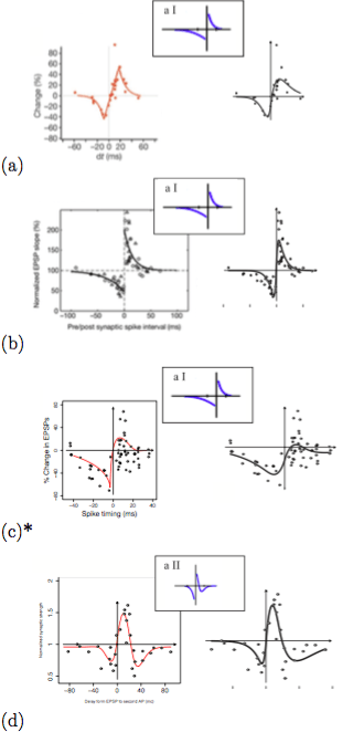
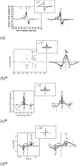
Figure 4. G-DHL-based regression of eight data-sets related to different STDP phenomena found in the brain. For each dataset, the graph reports the data from the source paper, the typology of STDP proposed by Caporale and Done (2008) to classify the data (small pictures), and the G-DHL regression curve. Image published with permission from PLOS from https://doi.org/10.1371/journal.pcbi.1006227

Given an STDP dataset, its regression with the G-DHL rule also allows the identification of the specific components of the rule and the events/derivative-parts underlying them. These events have a temporal profile that might resemble one of the biophysical processes causing the STDP kernel. This has a heuristic value as the profile represents a sort of identikit suggesting the possible temporal features of the causes of the STDP phenomenon to search with focused empirical experiments (Figure 5). The systematic fit of the STDP datasets considered in Caporale and Done (2008) also allowed the proposal of an updated taxonomy of different STDP phenomena based on their underlying G-DHL components.

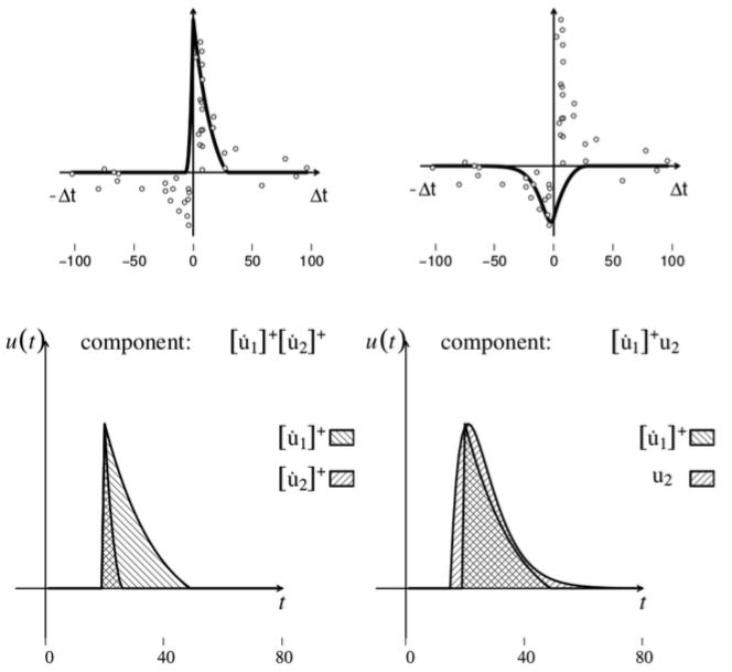
Figure 5. Top: two components of the G-DHL rule that best fit the classic STDP kernel found by Bee and Poo (1998) in hippocampus neurons, and shown in the top-left graph in Figure 4. Below: the temporal profile of the events generating the two components. Image published with permission from PLOS from https://doi.org/10.1371/journal.pcbi.1006227

Future research

Future work should test the idea of using the G-DHL rule applied to a specific STDP kernel found in the brain to heuristically guide the search of its possible underlying biophysical causes. Moreover, the rule might be used in artificial neural networks if one wants to take into consideration the relative timing of neural events as it happens in the brain. The rule thus represents a new tool for conducting research on learning processes both in the investigation of brain plasticity and in artificial neural networks.

These findings are described in the article entitled General differential Hebbian learning: Capturing temporal relations between events in neural networks and the brain, recently published in the journal PLOS Computational Biology. This work was conducted by Stefano Zappacosta, Francesco Mannella, Marco Mirolli, and Gianluca Baldassarre from the National Research Council of Italy (LOCEN-ISTC-CNR).