


Lake Erie is a vital resource to both the United States and Canada. It is the fourth largest of the Great Lakes and thirteenth in the world by surface area (25,655 km2) with a volume of 484 km3 and an average residence time of 2.6 years. The lake provides a potable water source for many cities including Buffalo, NY and Cleveland, OH; as well as a source of commercial fishing, industrial ports, leisure, transportation and agricultural irrigation.
The United States has already begun to see the effects of water shortage due to extensive agriculture and population growth in water limited regions. Being the fourth largest lake in the US, Lake Erie will undoubtedly play an even larger role in our economy and livelihood in the future. Therefore we must fully understand the variables that control the availability of this resource, which can be assessed through a detailed water balance of Lake Erie.
Despite the importance of Lake Erie, it appears that the most recent published paper conducting a detailed water balance of Lake Erie was Quinn and Guerra (1986), using data from 1940 to 1979. There have been vast changes in the use and management in Lake Erie’s water supply in the last thirty years. The most noticeable changes being from the 1960’s through the 1970’s when Lake Erie became extremely polluted by phosphorus runoff from agriculture, leading to lake-wide eutrophication, algal blooms, and fish death. Largely as a result of this case, the US Congress passed the Clean Water Act of 1972 in an effort to restore Lake Erie to its natural ecosystem. This act may have had profound effects on the hydrology of Lake Erie, depending on what action was taken to limit nutrient inflow. Fortunately, there are many agencies that monitor Lake Erie’s hydrology on a daily to monthly basis, providing ample data to update Quinn and Guerra’s interesting work in 1986.
The data Quinn and Guerra compiled from 1940 to 1979 for the water balance of Lake Erie produced fascinating results. They found that the mean precipitation from 1940 to 1979 was 5% higher than from 1900-1939, an increase of 37 m3 s-1. During this same period, the total water supply in the lake increased, as did the Detroit River discharge both of which were likely the result of the increased precipitation. They also noted a cooling trend starting in the 1950’s and lasting throughout the measured interval until 1979. These are just a few examples of how an updated water balance, looking at hydrological and meteorological data from 1979 to 2009, would help us understand the overall trends in the hydrology of Lake Erie.
Considering the importance of Lake Erie to the US, it is essential to understand and monitor the factors that influence its hydrology and available water supply. I will attempt to answer many of the open-ended questions posed in Quinn and Guerra’s paper as to the long-term trends in Lake Erie’s hydrology. I believe that the trend seen from 1940 to 1979 of increasing precipitation, lake water level, river flow, and decreasing temperatures will continue to 2009. This effect may largely be due to changing climate regimes; global warming seems like a viable mechanism for the increase in precipitation but one would expect an increase in temperatures as opposed to a decrease. Also, I examine how, if at all, the Clean Water Act of 1972 has changed the hydrology and water balance of Lake Erie.
Methodology
The basic equation used for a water budget of a lake simplifies down to Input – Output = Change in Storage. In this scenario, it is necessary to determine all inputs and outputs of water for Lake Erie. In addition, change in storage was calculated by taking the change in overall lake level from one month to the next and multiplying it by the surface area of the lake to get the overall volume of change in storage.
The inputs include inflow from the Detroit River, which is the only river source into Lake Erie and contributes significantly to the overall water budget. Additional inputs are precipitation falling on the lake, overland flow into the lake from precipitation on nearby land, and groundwater flow into the lake. The outputs include outflow through the Niagara River as well as the Welland Diversion. It also includes evaporation, consumption from the lake and groundwater outflow.
Consumption of water throughout the lake was measured only for a short period of time through the 1960’s, which measured an average of 48 m3/s (Quinn and Guerra, 1986). This value was used as a constant throughout the entire time series, and although a gross approximation, it amounts to less than 1% of the water leaving the lake. Groundwater flow into and out of the lake was not measured for Lake Erie and thus I do not take this into account in my calculation of change in storage. There is a good probability that this, like the consumption, would be a small fraction of the total water input or output. Also, the input of groundwater may act to balance the output of groundwater and thus cause little overall change in the storage of the lake.
Evaporation rates were needed in order to fully characterize the output of water from Lake Erie. GLERL collected temperature and wind speed measurements from Lake Erie from 1948 to 2000 and thus those measurements were used to model evaporation on the lake. Evaporation was calculated using the Mass-Transfer approach, which takes into account wind speed, surface topography, and both saturated and air vapor pressure. The lake temperature can be used to calculate saturated and vapor pressure through a relatively straightforward use of the Clausius-Clapeyron Equation. This was then used to calculate evaporation through the Mass-Transfer approach: E = KEua(ea-es), where KE is derived empirically. I was not able to use some of the more robust models such as the Penman-Combination Approach for evaporation since I did not have data on the heat budget of Lake Erie.
Data
The National Oceanic and Atmospheric Administration (NOAA) runs the Great Lakes Environmental Research Laboratory (GLERL). The GLERL monitors hydrology and hydraulics data for all of the Great Lakes, including stream flow, connecting channel flow, lake evaporation, evaporation, water temperature, and water quality assessments. It also records precipitation on and around the lakes, temperature, runoff and lake level. I used this data supplied by GLERL to conduct a current water budget for Lake Erie. The Detroit River accounted for approximately 80% of the inflow into Lake Erie, while the Niagara River accounted for nearly 86% of the outflow from the lake. The average lake level throughout the 100-year record was 174.1 meters.
| In (m3/month) | % of In | Out (m3/month) | % of Out | ||
| Detroit River | 1.39×10¹⁰ | 80.1 | Consumption | 1.26×10⁸ | 0.7 |
| Precipitation | 1.89×10⁹ | 10.9 | Niagara River | 1.51×10¹⁰ | 85.8 |
| Runoff to Lake Erie | 1.56×10⁹ | 9.0 | Welland Division | 4.08×10⁸ | 2.3 |
| Evaporation | 1.97×10⁹ | 11.2 | |||
| Average Lake Level | 174.1 m | ||||
Bathymetry
Throughout the 100-year record, the maximum lake level recorded is 175.04m and the lowest is 173.17m, a difference of 1.87 meters. As you can see from the figures below of the bathymetry of the lake, it appears that there may be an inherent error when calculating water volume by multiplying the values by the surface area of the lake. As the lake level rises and falls, the surface area of the lake changes and this needs to be quantified or explained. After further research, it is clear that the effect of changes in lake levels on the surface area of Lake Erie is assumed to be negligible. As the water drops it does cover less surface area, however, the large size of Lake Erie mitigates the effect of changing water levels on surface area. In the USGS Scientific Investigations Report 2004-5100 on the Great Lakes Water Balance, they discovered that a change in lake level resulting in an average loss or gain of approximately 500 ft of shoreline would be needed to change the area of the Great Lakes by 1%. For this reason, change in surface area of Lake Erie was not taken into account when quantifying the change in storage.
As a qualitative assessment of the change in surface area due to the change in lake level, one may assume the relative direction and magnitude of variation in this estimation. The low levels in change in storage are most likely overestimated since the surface area would be slightly less, and therefore the troughs in the change in storage graphs may be in reality slightly shallower. On the other hand, the high values in change in storage are most likely underestimated, since the lakes surface area would have increased slightly. This would mean that the peaks in the change in storage figure, in reality, should be more pronounced.
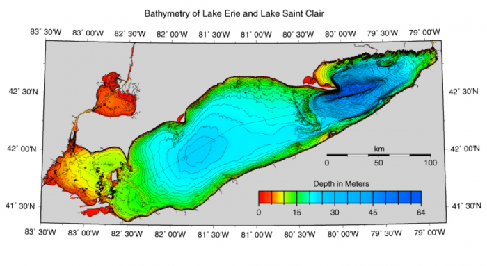
Bathymetry of Lake Erie
Change in Storage via Lake Level
Below is the calculated change in storage using the monthly lake level data. One month’s lake level was subtracted from the previous month’s lake level and multiplied by the total area of the lake (25,655 km2). This gave a running series of the changes in storage for Lake Erie. It appears that from around month 700 (1958) onwards there is less variation in the data, maybe suggesting that the lake became more regulated by hydroelectric dams and/or water use.
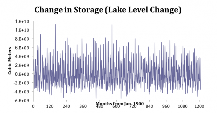
Change in Lake Erie water level
Due to a large number of data points and the difficulty of teasing out valuable information about the change in storage from the graph above, a running sum of the change in storage was calculated to show long-term variation. Below is the running average of the change in storage for Lake Erie. One can notice that the overall change in storage increases from 1900 to 2000. Also, there are several low points, namely at around months 400 and 800, coinciding with 1933 and 1966.
The dust bowl occurred in 1933 so that may be the cause of the dramatic decrease. There are also several drastic increases in the change in storage, the most prominent at approximately month 350, corresponding to the flooding of 1929. In addition, one can see three prominent cycles in the change in storage, which appears as longer trends of rising and falling of the change in storage. To better see this trend it is useful to look at the 5-year running mean of the sum of the change in storage. This clearly shows that there is a 30-year variability, visualized as “humps” in the sum of the change in storage. This trend was hidden in the initial change in storage plot but is clear in the running sum.
There appears to be a 30-year regime that repeats itself throughout the record, although it is hard to say how long this regime has been present since we only see 100 years of the record. One can also see the major climactic events in North America throughout the last century in Lake Erie. The Dust Bowl, in the 1930’s, is clearly evident in addition to the 1929 flooding events, which took place right before the Dust Bowl. During the 1960’s Lake Erie became widely eutrophic, killing vast amounts of fish and turning the lake nearly anoxic. As a response to this eutrophication, Congress passed the Clean Water Act around 1970, which implemented regulations in the usage and dumping of sewage or fertilizer into the lake. This event is marked on the change in storage figure, and corresponds to a dramatic increase in lake wide storage, alluding to the success of this act in helping to regulate the Lake’s resource.
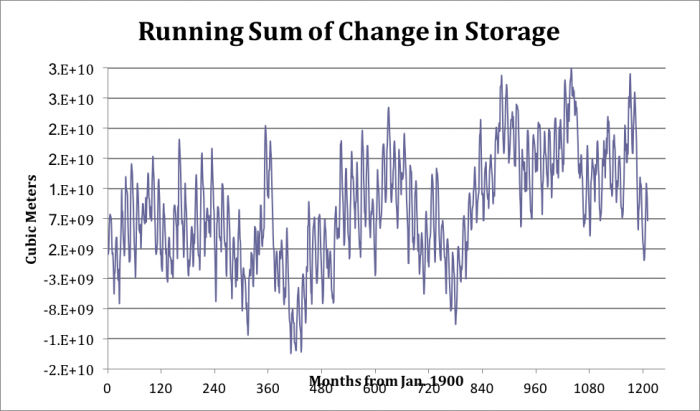
Running Sum of Change in Storage
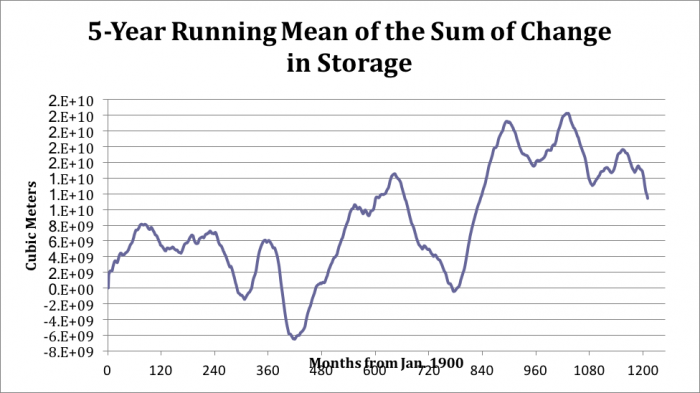
5-Year Running Mean of the Sum of Change in Storage
Change In Storage (Input-Output)
Change in storage was also calculated via the method described earlier by subtracting the output from the input to Lake Erie. The input is the Detroit River input + precipitation + runoff into the lake + base flow into the lake. The output is evaporation + Welland Division output + Niagara River output + base flow out of the lake + consumption. One caveat is that this method was only applicable from 1948 to 2000 as opposed to 1900 to 2000 for the lake level change method. This is because there are only temperature and wind speed measurements (which were used to calculate the evaporation rate) for Lake Erie from 1948 to 2000. As you can see below it is very much the same as the change in storage calculated by the change in lake levels.
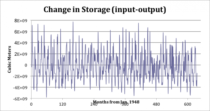
Change in Storage (input-output)
Melting Season Precipitation
A useful approach to looking at the causation of the fluctuations in change in storage may be to look at the temperature variations for each given month throughout the record. Lake Erie is partly supplied by meltwater from snow covering the region and thus a change in the temperature from year to year may indicate the magnitude and temporal variability in the water reaching Lake Erie.
The figure below shows the monthly changes in temperature from 1948 to 2005, assuming that the majority of the melting occurs from January to April of each given year. The time series is somewhat hard to delineate long term trends or significant fluctuations. The most significant change is the decrease in temperatures throughout each month from around 1975 to 1978. This period, when looking at the sum of the change in storage corresponds to one of the peaks and where it starts to descend. This could indicate that the reason for the peaking of the change in storage, and subsequent decrease, is the unusually cold temperatures limiting the snow melt from reaching the lake.
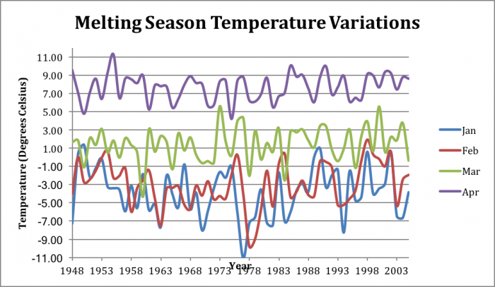
Melting Season Temperature Variations
Wavelet Analysis
The use of a Morlet Wavelet can indicate signals of periodicity in a data series that are not visible to the naked eye. Below are the wavelet spectra for the change in storage calculated from lake level change as well as input – output methods. Both show similar trends, which is expected since they ideally should be exactly the same as one another. On both graphs there is a strong yearly (12 month) periodicity that runs throughout the entire record, the black contour line that surrounds the red band at 12 months is the 10% significance level, indicating that this periodicity is in fact significant. Also, when looking at part C, the Global Wavelet, the confidence interval indicates that 12 months is the only significant periodicity in both of the spectra. This is expected since there are seasonal inputs of melt water that supply much of the total water input to the lake each year.
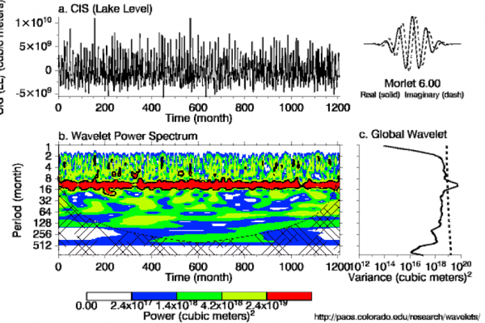
Fig: (a) CIS (Lake Level). (b) The wavelet power spectrum. The contour levels are chosen so that 75%, 50%, 25%, and 5% of the wavelet power is above each level, respectively. The cross-hatched region is the cone of influence, where zero padding has reduced the variance. Black contour is the 10% significance level, using a white-noise background spectrum. (c) The global wavelet power spectrum (black line). The dashed line is the significance for the global wavelet spectrum, assuming the same significance level and background spectrum as in (b). Reference: Torrence, C. and G. P. Compo, 1998: A Practical Guide to Wavelet Analysis. Bull. Amer. Meteor. Soc., 79, 61-78.
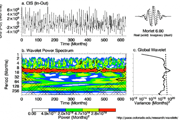
Fig: (a) CIS (In-Out). (b) The wavelet power spectrum. The contour levels are chosen so that 75%, 50%, 25%, and 5% of the wavelet power is above each level, respectively. The cross-hatched region is the cone of influence, where zero padding has reduced the variance. Black contour is the 10% significance level, using a white-noise background spectrum. (c) The global wavelet power spectrum (black line). The dashed line is the significance for the global wavelet spectrum, assuming the same significance level and background spectrum as in (b). Reference: Torrence, C. and G. P. Compo, 1998: A Practical Guide to Wavelet Analysis. Bull. Amer. Meteor. Soc., 79, 61-78.
Comparison of two Change in Storage methods
I compared the change in storage calculated from the lake water level and from subtracting the outputs from the inputs for Lake Erie. Surprisingly they match up almost identically when you plot them both together, indicating that both methods appear to be accurate. This also indicates that the absence of a value for the base flow in and out as well as the approximation of consumption may not have played a large role in the change in storage for the lake. It also verifies that the measurements are accurate enough to correlate closely with the observed fluctuations in lake level.
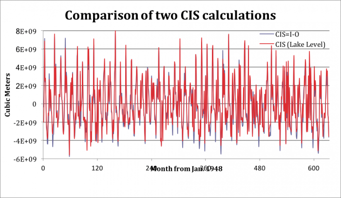
Comparison of two CIS calculations
Lastly, I plotted the two changes in storage against one another in order to compare the two and see quantitatively how well they correlated with one another. As expected, they correlate extremely well, with an R2 = 0.94. The slope of the line is also nearly 1, at 0.98, which indicates that there is practically a 1:1 relationship between the two methods as would be expected since they ideally measure and record the same information. Lastly one can see that there is no skew in the relationship depending on whether there was a positive or a negative change in storage, indicating that there was no instrumental or measuring bias due to an increase or decrease in change in storage.
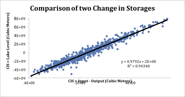
Comparison of two Change in Storages
Conclusion
A significant amount of information has been gained through this water balance of Lake Erie. Firstly, the measurement collection conducted by GLERL should be commended, as the two methods of calculating the change in storage were so closely correlated. It was also shown that Lake Erie has an approximately 30-year cyclicity in its water storage, giving insight into the long-term trends that the US government can expect to see in Lake Erie. In addition to the 30-year cyclicity, it was shown that Lake Erie has a yearly periodicity that is most likely influenced by the melting of snow accumulation in spring of each year.
The Lake also recorded major climatic variations in addition to the onset of regulations such as the Clean Water Act in the 1970’s. Lake Erie is an important part of the United States economy and well being, and it is encouraging to have the resources to look at the lake through a water balance to better understand the hidden messages that lie within the measurements. These will inevitably be useful tools in determining how we will use and conserve this resource in the future.
References
- National Oceanic and Atmospheric Administration, Great Lakes Environmental Research Laboratory. Used for raw data:
- Neff, Brian P., and Nicholas, J.R., 2005, Uncertainty in the Great Lakes Water Balance: U.S. Geological Survey Scientific Investigations Report 2004-5100, 42 p.
- Neff, B.P., Killian, J.R., 2003. The Great Lakes Water Balance: Data availability and annotated bibliography of selected references. USGS. Water Resources Investigations Report 02-4296.
- Torrence, C. and G. P. Compo, 1998: A Practical Guide to Wavelet Analysis. Bull. Amer. Meteor. Soc., 79, 61-78.
- Quinn, F.H., Guerra, B., 1986. Current perspectives on the Lake Erie water balance. J. Great Lakes Res. 12, 109 – 116.
Related Posts
 Duck-Billed Dinosaurs Uncovered In Aniakchak, Alaska
 Cryptic Diversity In Vietnam’s Limestone Karst Habitats
 An Improved Method To Remove Debris From Cyst Nematode Egg Suspensions And Computer-Aided Technologies For Egg Counting
 The Footprints Of Urbanization, Industrialization, And Agriculture On River Beds: Heavy Metal Contamination Assessment And Source Identification In River Sediments In Eastern China
 Aging Dolphins Via Pectoral Flipper Radiography
 Glycoalkaloids In Potatoes: The Effect Of Biostimulants And Herbicides