


Hundreds of thousands of asteroids are orbiting our Sun with different orbital periods according to their mean distance to the Sun, or semimajor axis. All of them are gravitationally perturbed by the massive planet Jupiter.
The cumulative perturbations of Jupiter, and, to a lesser extent, other planets, generate a slow orbital evolution. Sometimes the asteroids’ orbital periods are in a simple fractional relation with the orbital period of Jupiter. In this case, this synchronicity accumulates a strong orbital perturbation in the long term that generates a peculiar orbital evolution. This phenomenon is known as orbital resonance.
The first evidence of orbital resonances in the population of asteroids was obtained by Kirkwood in 1866. He found evident gaps in the distribution of the semimajor axes of the asteroids exactly there where the orbital periods were simply related to Jupiter’s orbital period. For example, there is a gap at 2.5 astronomical units (au) from the Sun where the corresponding orbital period is 1/3 Jupiter’s orbital period. In modern language, we refer to this situation as the 3:1 resonance with Jupiter. We now know that this gap is due to a strong dynamical instability that appears inside this resonant motion but not outside of it. In the 90s, a large population of trans-Neptunian objects started to be discovered and as discoveries increased an analog pattern of resonances, with Neptune becoming evident in the trans-Neptunian region.
For decades, astronomers tried to understand this dynamical mechanism that not only generates gaps in the population of objects but also concentrations. For example, the Hildas is a concentration of approximately 4500 asteroids evolving inside the 3:2 resonance with Jupiter, which means their orbital period is 2/3 the orbital period of Jupiter. In analogy, there is a stable population of objects concentrated in the exterior 2:3 resonance with Neptune. Pluto is the most popular object of this population which has an orbital period 3/2 times the orbital period of Neptune.
The other very relevant population of resonant objects are Jupiter’s Trojans, consisting of approximately 5500 objects that are in the resonance 1:1, which means they share the same orbital period of Jupiter. At present, we know about objects evolving in resonances with almost all planets of our solar system. The stability of the resonant motion is defined by long-term effects that occur inside each resonance, and they are different for each resonance. For example, inside the 3:1 resonance with Jupiter, the long-term dynamics excite the eccentricity to almost 1, transforming the asteroid in a projectile that will collide with other planets or with the Sun.
Why do some resonances show up, but for others, there are no dynamical traces? Astronomers found that each resonance has an associated “strength”: strong resonances generate strong dynamical effects (gaps or concentrations) and they cover larger regions in the space of semimajor axis. Weak resonances do not generate notable orbital evolutions and they operate in a very limited region in the space of semimajor axis. For example, the strong resonance 3:1 with Jupiter affects all asteroids with the semimajor axis between 2.44 and 2.56 au, while the weak resonance 1:2 with Mars affects only asteroids with the semimajor axis between 2.417 and 2.419 au.
Analytical theories allowed a very complete description of the resonances, but under the restriction of near-coplanar orbits for the considered planet and the small body. These theories showed that the resonance’s strength is proportional to the mass of the planet that generates the resonance and also proportional to the orbital eccentricity of the resonant small body. That means that for larger orbital eccentricities the resonances are wider in the semimajor axis. For large enough eccentricities the resonances are so wide that they overlap constituting a continuum of resonances, generating a chaotic behavior.
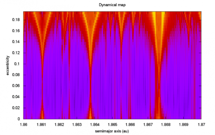
Figure. Numerical exploration of the dynamical evolution of 20.000 test particles with eccentricity between 0 and 0.2 and the semimajor axis between 1.86 au and 1.87 au. Dark or blue regions correspond to negligible orbital changes and red and yellow regions correspond to large orbital changes. All orbital changes in this very thin slice in semimajor axis (only 0.01 au) are due to a “forest†of resonances with Jupiter and Mars principally. The domain of the resonances grows with the eccentricity. Image published with permission from Tabare Gallardo
But, what happens when the asteroid has some orbital inclination? There are several cases of small bodies with large inclinations, greater than 60 degrees, for example. More interestingly, there are hundreds of objects with such high inclination that, in fact, their directions of revolution around the sun are contrary to the direction of revolution of the planets. We call them retrograde objects, and they have orbital inclinations between 90 and 180 degrees.
What happens to the resonant motion when the orbital inclination is large or retrograde? Does it make any sense to think about resonances for retrograde orbits? No satisfying theories were presented up to now for these very inclined orbits because the complexity of the algebra involved does not allow us to find simple answers. Serendipitous evidence of the relevance of retrograde resonances came from the numerical exploration of the dynamical evolution of comets. In numerical integrations of comets that show their possible future evolution in timescales of millions of years, it was found that, frequently, they become captured in retrograde resonances, especially in resonances exterior to the planet of the 1:N type, that means 1:2, 1:3, and so on.
An astonishing discovery paints the scene of the relevance of retrograde resonances: in 2015, the object 2015 BZ509 was found to be co-orbital with Jupiter (resonance 1:1) but with an orbital inclination of 163 degrees, which means orbiting around the Sun contrary to the orbital direction of Jupiter. They do not collide because the orbit of the asteroid has some eccentricity, and they are synchronized, avoiding catastrophic encounters.
An approach to the study of the high-inclination resonant orbits was proposed by Gallardo (2019, Icarus). The idea is to numerically compute the resonant perturbations assuming that the object and the planet have fixed orbits. The method is very efficient in providing strengths for thousands of possible resonances in minutes using a standard computer. It is also rigorously valid for arbitrary orbital eccentricities and inclinations. The principal result obtained exploring the resonances using this method is that for high inclination or retrograde orbits, all resonances at some point become weak and they can break the resonant motion, except for resonances of the type 1:N, including the 1:1 resonance, for which their strength is always large, so in timescales of millions of years they become reservoirs of resonant retrograde objects.
In recent years it became evident that in extrasolar systems, in the asteroid belt, and in some satellite systems, there is another type of orbital synchronicity: three body resonances (3BRs). The first documented case of a 3BR was due to Laplace and it involves the orbital motion of the Jupiter´s satellites Io, Europa, and Ganymede. The orbital period of Ganymede is exactly twice the orbital period of Europa, and the orbital period of Europa is exactly twice the orbital period of Io.
This type of 3BR can be considered a superposition of two-body resonances (2BRs) or a “chain” of 2BRs. Chains of 2BRs are observed in particular in extrasolar systems and can be explained by captures in resonance generated by the migration that the planets experience in the last steps of planetary formation. In fact, our planetary system is very close to chains of orbital resonances. But there is another type of 3BRs that do not involve 2BRs and occurs when the orbital period of an asteroid can be expressed as a linear combination of the orbital periods of two arbitrary, not mutually resonant, planets. Looking for this kind of “pure” 3BRs, Smirnov et al. (2018, Icarus) found tens of thousands of asteroids evolving inside 3BRs with two planets, mainly the pair Jupiter-Saturn.
Three body resonances are very weak and they cover very thin regions in semimajor axis, some 0.001 au or less. Nevertheless, they are numerous and they generate large accumulations of asteroids transitorily trapped in resonant motion. This can be seen if we plot a histogram of the semimajor axes of the known asteroid population.
Orbital resonances are not an exotic mathematical singularity; they have a clear physical meaning and an indisputable dynamical effect: they explain the orbital architecture of the exoplanetary systems, and they sculpt the distribution of minor bodies in our Solar System generating voids and reservoirs.
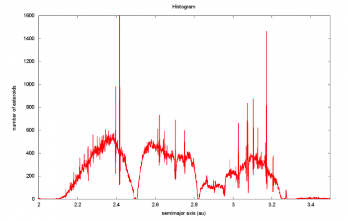
Figure. A number of asteroids per 0.001 au between 2 and 3.5 au in the region between Mars and Jupiter. The gaps are due to strong resonances with Jupiter and each peak is due to weak two-body orbital resonances (mainly asteroid-Mars) or three-body orbital resonances (mainly asteroid-Jupiter-Saturn). Image published with permission from Tabare Gallardo
These findings are described in the article entitled Resonances in the asteroid and trans–Neptunian belts: A brief review, recently published in the journal Planetary and Space Science. This work was conducted by Tabaré Gallardo from the Instituto de Física, Facultad de Ciencias.
Review:
References:
- https://www.sciencedirect.com/science/article/pii/S0019103518300423
- https://www.sciencedirect.com/science/article/abs/pii/S0019103517300386
Website:
Related Posts
 Search For Life: How Organisms On Earth Help Us Understand Space Environments
 The Existence of Complex Life In The Universe May Be Rarer Than Previously Thought
 From Laboratories To Space: Experimental Organisms Contribute To Space Research
 Early Human Settlement On Mars By Sheltering Them In Excavated Underground Structures Due To Harsh Climate And Hazardous Solar And Galactic Cosmic Rays
 Circuit QED Controlled To Implement Quantum Computers
 Dark Matter Meets Einstein’s Equivalence Principle: A Tale Of Two Particles